Part 4 of our Excel Guides series. Read Part 1, Part 2 and Part 3 here.
Another frequent request from our clients when dealing with data is “how do you merge information from two separate files?”. This is usually matching responses to an email campaign back to the customer data, or matching up customer details to purchases.
The simple answer I use is the formula VLOOKUP. This simply looks at the field of the first record (email in our example) and looks it up in the full column of email addresses in the other file. When it finds a match, it looks along the row in the second file and picks up the new data and copies it into the first file next to the email address. It then moves on to the second record and does the same, right through to the end of the list. If it doesn't find a match it just returns an error against that record (#N/A in Excel's "easy to understand" language).
We'll take it one step at a time.
Step 1 - Put both files together
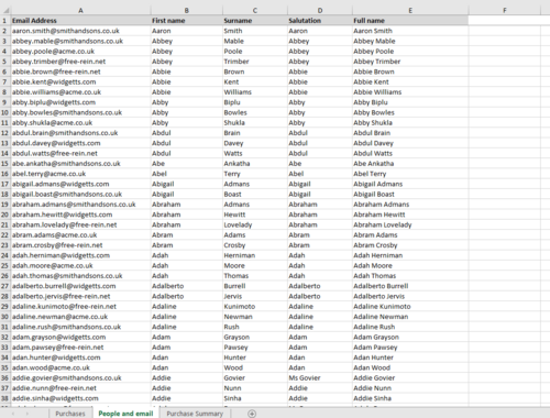
You'll find it easier if you have both sheets of data in one file. Open both files. On the sheet tab of one of them, right click, choose Move or Copy. In the drop-down menu at the top, choose the other file, tick Create copy and click OK. You now have a file with two data sheets. Give them sensible meaningful names. In our example we have People and Purchases.
Sort the People sheet in alphabetical order of email and make sure it is the left most column.
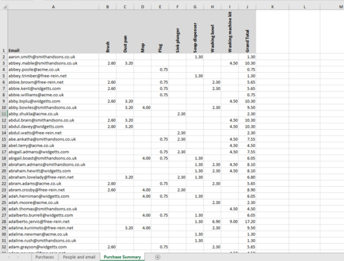
Sort the Purchase sheet in the same order (this one was created by a Pivot Table in an earlier blog). This is not vital but it speeds the whole matching process up and is kinder to less powerful machines.
Step 2 - Calling up the Function
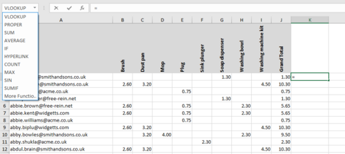
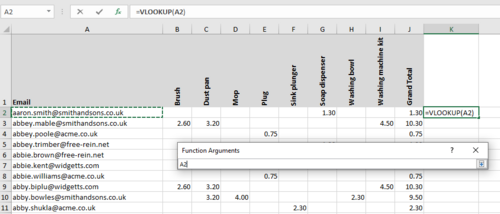
Put the cursor in the first blank column to the right of the first email address to be matched (K2 in our example). Insert an equal (=) sign. You will see a drop-down menu just above the A column - it has a white background. Drop the list down and look for VLOOKUP. If you can't see it in the list choose More Functions and a window pops up. Select the Lookup & Reference category in the drop down and then VLOOKUP in the list that appears under that.
Step 3 - VLOOKUP Explained
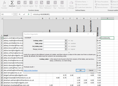
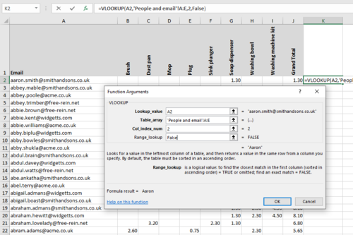
You get a new pop up which is the template guide to using VLOOKUP. There is an explanation of each step. The four fields are:
Lookup_value – this is the first data element you want to find. In our case it is the email address in A2.
Table_array – these are the columns in the other sheet that hold the email addresses to be matched and the data to come over.
Col_index_num – this is just the number of the column that holds the data to be brought to that field.
Range_lookup – True or False. True finds the first closest match, False finds an exact match only.
Step 4 - Filling in the fields
Click on the arrow next to the Lookup_value field.
Then, click on the email address in A2 and click on the arrow again. This is the first field to match. The system will automatically step down the column until it gets to the end. If you wanted to search across a row you won't be surprised that you need to use the HLOOKUP function!
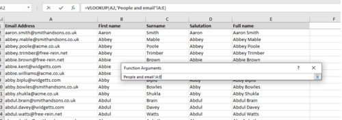
Now click the arrow next to the Table_array field. Navigate to the other sheet, in our case the Purchases, and select the rows that have the data to be matched and the data to be brought across. In our example we are using the email column to match and we want to bring over the first name, surname and full name. So we need columns A:E.
Click the arrow again to go back to the function template pop-up. Now type in ‘2’ in the Col_index_num field. This is the second column along in the range you have chosen and in our example is the First name column. This is the data that will be brought across when a match is found. Finally, in the last field type ‘False’ as we only want exact matches in this case.
All done so hit OK.
Step 5 - Replicating the formula
The formula appears as =VLOOKUP(A2,'People and email'!A:E,2,FALSE)
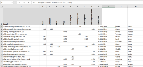
However, we are going to copy this and use it in column L and M to bring across the Surname and Full name (columns C and E in the People sheet). If we just cut and paste though, Excel would adjust the formula to maintain the same mapping which would be the wrong look-up fields. So, change the formula to add the $ sign in against the field references that do not change. =VLOOKUP($A2,'People and email'!$A:$E,2,FALSE)
Now copy the new formula to L2 and M2. The only item that needs changing is the Col_index_num to identify the surname (C column - number 3) and Full name (D column - number 4). When that is done, copy those three fields down the column. The quickest way is to select the field and then double click on the black square, bottom right of the select area.
Give the columns meaningful names and you have your complete data!

